So far page is under construction and serves mostly just as my notesheet, cause I would get otherwise lost in these notes without links… – this part of page is still semi-official – semi home is here – Sequencing, resp. here for Pd.
Page is looking for proper shaping – 1) Using single exponent then polynomials (w/ regard to hyperbolas and goniometric) and then 2) Bezier shapes.
Content points preview
Curve incubator I. a) Power/ Root (basic curves), Logarithm b) Trigonometric fncts. c) Ellipse, parabolic, hyperbolic fnct. II. Approximation (Interpolation) of polynomials
Jamming and interpolation as math and music bridge
Music and math bridge here is jam (jamming) – rigid structures going faster or slower. One of the key techniques to create curves or waveforms is interpolation respectively extrapolation. That is actually what jamming or modulation of ADSR parameters is (in its core) about..
Coding and Algorithm I. Algorithm and Attractors – Thue-Morse sequence – Markov Chain – Group theory – Hop-along attractor
II. Coding Meshing
I-a. Exponential: Power, Root and LOG
For interpolationone needs non-parametric equations – two or more variables: while DAWs typically have one variable y andstatic change (so not really changing)) timeline – x,so interpolation is directly possible only via approximation – tough it is limited, it has some advantages – see Chapter II. However interpolation can be used indirectly thru XY pad – see: Non-parametric equations.
Logarithm
– ..
Power/ Root: Advanced Envelope and Curve module like curves
Modulate envelope´s ADSR parameters (only way to do curves in DAW) has its downsides: 1) U will never really see the shapes and timing u ve made and never get a feel for them. 2) Changing ADSR parameters in the envelope will not properly change note length if desired.
—————————————————- Grid´s Curve module – as u can see in oscilloscope is just use exponent of 1 to 4 and that´s it. ADSR Envelope using adding Power and Root and then dividing it by two – no way to change the balance, same way like in Curve module, which is strictly curved around one gravitated center point.. You see, this is what they make you give. —————————————————-
And u can check 4 yoursel in - here - In Tracks Envelope and Curve module it is display, what these are doing..
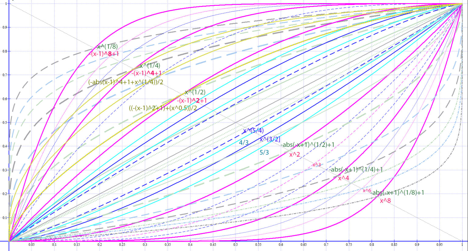
Curvature based on single exponent
As u can see, there are much more options compare to standard DAW/Synths – giving u some control over the curvature which can be musically adjusted in steps similar to steps/ half-steps in notation (midi notes) and also lean it out of one gravitated point, because Curve module does not take into account dashed lines and Envelope is using 50:50 mix of dash and full lines..
1a) Convex (bend down) Attack Power x^2 – 4 – 8 – (16 – not on pic tough) represent (like in pitch) same additional amount of extra curvature – curvature that is leaned to start: x^8 exponent peak deviation happen before crossing x ^-1 line – it actually stay on 0 level till almost 1/2 its range. – its Root counterpart -abs(-x+1)^1/2 – 1/4 – 1/8 + 1 – is on the other hand leaned to end: its 1/8 exponent peak deviation happen after crossing x -1 – almost at the end of its range it is still just on 0,5 level. 1b) Similarly but inversely Concave (bend out/up) attack Power -(x-1)^2 – 4 -8 +1 – are equal steps leaned to end: ^8 exponent peak deviation happen after crossing x -1 – it actually stay on max level almost from 1/2 its range. – its Root counterpart x^1/2 – 1/4 – 1/8 – is on the other hand leaned to start: ^1/8 exponent peak deviation happen before crossing x -1 – almost still at the start it already in its 0,5 level value. 1c) if we add Power and Root and divide it by 2 – like: ((-(x-1)^2+1)+(x^0.5))/2 – we will get balanced shape, which is in Bitwig used for ADSR in range from 0 to 4. – this curves are shown only in convex shaping as yellow curves w/ grey dotting in ^2-3-4 exponents, but obviously u can make it same way w/ any exponent.
Limitation of these curvese
– despite advantages and fair range of use, it also brings some limitations. Bottom line is, that these curves should go hand in hand w/ regular Bézier shapes to be fully useful. 1) x^4 actually stays 1/4 of its time on 0 level – it is actually just same as x^2 run 25% faster. – u can partly solve/ avoid this issue using 3 segments in one slope – but then when u will be moving w/ center of gravity as demonstrated in Enseq device, u will be left out with long straight lines. – I found it rather undesirable, since I
2) One would still like to know, how is the speed changing at particular points – how would be an orthogonal line at particular points at the curve tilted – and that is exactly what calculus is and that is exactly and very unfortunately not an exactly easy thing… see Chapter II. Tough u can partly solve it by subtracting/ adding x^1 curve – this will show overall offset.
3) It not easy to keep shape proportionate – is lacks of continuity of the curves which is as u can see in Chapter II again just a nasty calculus – derivation of 1 and 2 degree particularly…
Even tough this approach is simplistic, it has few aces in sleeves – it is bloody predictable and mess-up able.
– exponents can be modulated as keys: more on Enseq-scale.
Bitwig PHASE like clocking in Plugdata
– matsicaly (mathematicaly/ musicaly) jam is defined by acceleration – can be speed with km/ h in sec, in music it is described similarly by Hertz per sec resp. change in cents, intervals, note per sec.
In BW u can change the phase speed by offsetting w/ Shifter or directly w/ Scaler – both methods will have its limitation: most notably new phase speed has to be in integer ratio of former phase and have to changed in the time-span of particular phase – BWlimit.
While BW can made some shapes, timing is tricky, since Phase is hardwired to one of the standard notation 1/2-64.
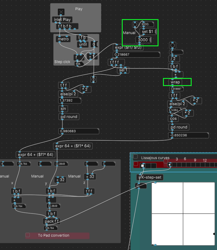
In Pd once make classical clock (Lgreen), adjust its normalized 0-1 time in ms as desired (Lred) and make vary speed tracks – Phase offsets w/ wrap module (Rpic).
Chirp .. one of the fnct that count w/ varying speed – resp. constantly varying speed is call chirp – it can do linear change, but also exponential and hyperbolic. But I guess I am not the only one not happy that it use calculus.. There is some quadratic phase signal – that counts with: c – rate of change θ(0) – phase offset (initial phase) than .. sin( 2pi(c/2t + f0t) )
I-b. Hyperbolic,Parabolic and Elliptic fncts.
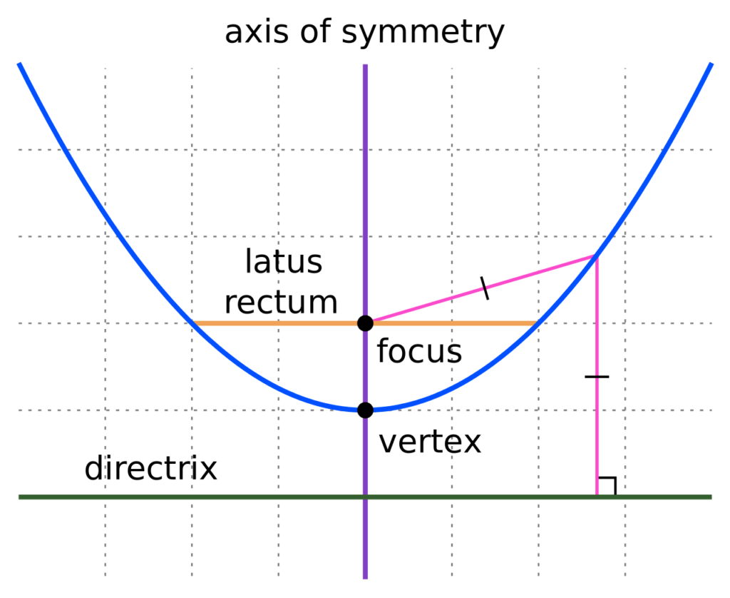
– while sin is projection of circle into plane, ellipse, parabola, hyperbola can be similarly projected – see chapters Kepler rotator and Planes. – key characteristic of these lines is focus (and that is also why they are used in optics)) – focus is point to which distance from any point to curve is in same ratio like the distance to directrix – for parabola (Rpic) it is 1: so distance is always the same (see more to it on this subpage).
Eccentricity
Lorem ipsum dolor sit amet, consectetur adipiscing elit. Ut elit tellus, luctus nec ullamcorper mattis, pulvinar dapibus leo.
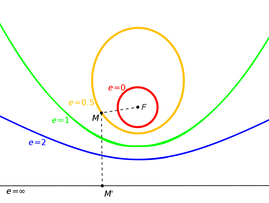
Like in inter/extrapolation one moving with poles, with eccentricity one moving with center of the circle. e < 1 – Ellipse e = 1 – Parabola e > 1 – Hyperbola
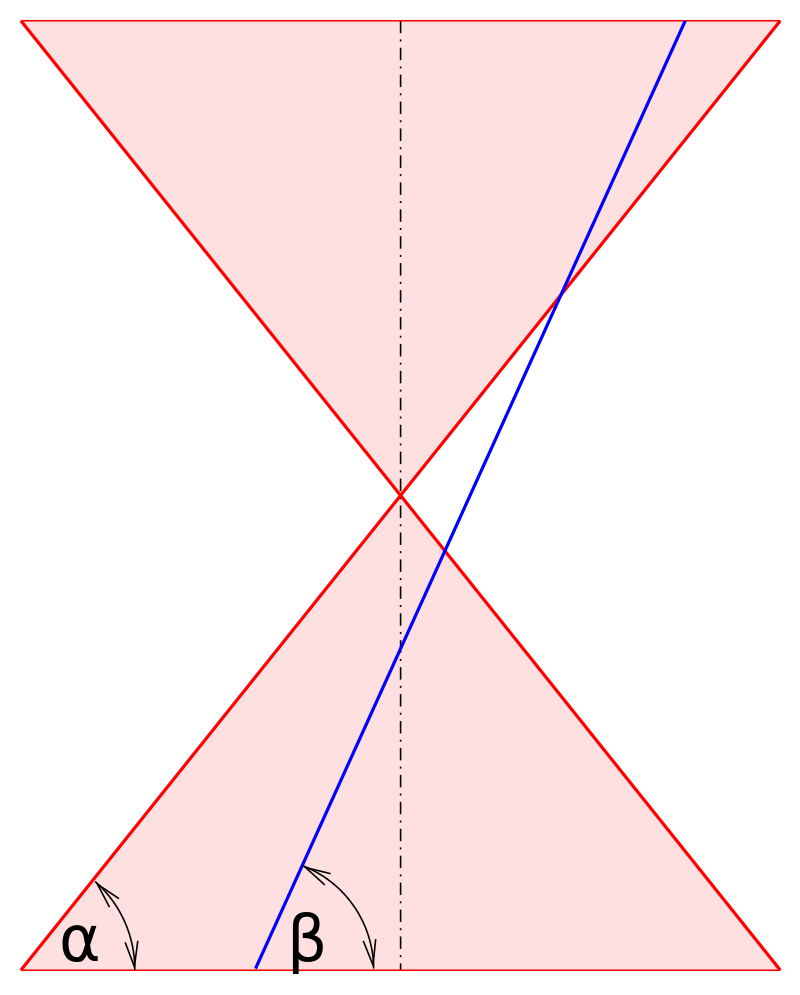
Angular eccentricity AE can be written in terms of eccentricty per se or with b/a ratio.
Para
Angular eccentricity AE can be written in terms of eccentricty per se or with b/a ratio.
While sin wave is just simple projection of unit circle it also mimic change of dimension from plane to space – or we can say putting two planes orthogonally (adding 90° axis) – or we may say one step higher dimension: linear orbit of the object appears to be slowing down and increasing the speed. It is not just a concept, interesting is, that soundwaves, electromagnetic waves, structural mechanics, earthquake waves are based on same principles.
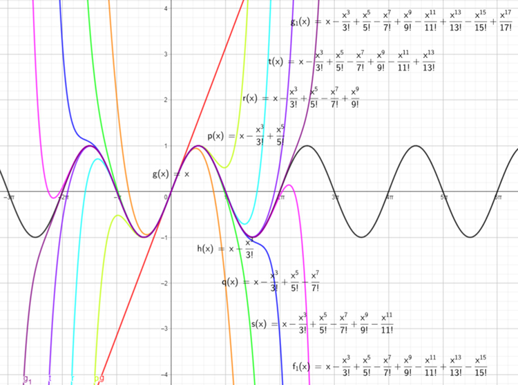
Derivation of sin
– sinus can be expressed w/ exponents (polynomials) w/ Taylor series – 16 orders give one full cycle (Lpic): see in Calculus, chpt. Taylor series – here. Red is 1. order, org – 3, l-green – 5, ..
– in chapter Quantum mechanics oscillator u can see it is based on Simple harmonic motion (SHM) – define by sin wave (ignoring gravity, friction, dumping/ driving forces) and describing also motion of simple harmonic oscillator – which u can get in unit circle analogy by looking at 3D circular motion from outside on its orbit 2D plane (Rpics). – Complex harmonic motion (CHM) – taking into account gravity, friction..
SIN & COS making CYCLE
– w/ sin on x and cos ony resulting line creates circle. – it is actually special case of Lissajous curve – seehere. – circle and first Lissajous shapes are pretty oldschool, but u can get Besace, Lemniscate of Bernoulli and bunch of non-parametric shapes.
Envelope base on sin
I. Night/ Winter (cold) semi-cycle (0-180°) 1. q: 0 – 1/4 (0-90°) rise equilibrium – maximum 0h Pisces (Night) – 6h (Taurus) In env. Nïght: Rise (1. q) – Attack In note: Kick/ subs dominated – usually longer.
Deviation from triangle – constant speed 0 – min (0) deviation max acceleration 1/8ish – max deviation average (constant like speed)
2. q:1/4 – 1/2 (90-180°) fall maximum – equilibrium 6h Taurus – 12h (Virgo) In env. Morning: Sustain + Release In note: Snare A (noise dominated)
Deviation from triangle – constant speed 1/4 – 0 deviation max deceleration 3/8ish – max deviation average (constant like speed)
II. Day/ Summer (Hot) semi-cycle (180-360°) 3. q: 1/2 – 3/4 inversed rise equilibrium – minimum 12h Virgo – 18h (Scorpius) In env. Afternoon: Rise2 In note: Kick/ subs dominated
Deviation from triangle – constant speed 1/2 – 0 deviation max inverse acceleration 5/8 – max deviation average speed 4. q: 3/4 – 4/4 inversed fall – minimum equilibrium 18h Scorpius – 24h In env. Evening: Fall2 In note: SnareB
Deviation from triangle – constant speed 3/4 – 0 dev. max inverse deceleration 5/8ish – max dev average speed 4/4
II. Bezier shapesw/ approximation-interpolation based on vectors
– polynomial are most flexible – more flexible then trigonometric fncts or vectors: which is basically only way to get shapes. – so called Bezier curves used in DAW are not that much Bezier curve (if at all)).. – Bezier curves (BC) were introduced in 60s with French designer Bezier, who worked for Renault and are generally based on different principle.. vectors, while in DAW shape is mostly made by simple exponent, but same principle can be used on more advanced non-parametric curves. But modulation of ADR(S) parameters loosely uses vector based interpolation, but modulates only one point – so it is smth between LERP (linear interpolation) and can be (with raised eyebrow) considered as simpler form of quadratic curve, while typical shapes inCAD(computer-aided design) used cubic shaping – using three points.
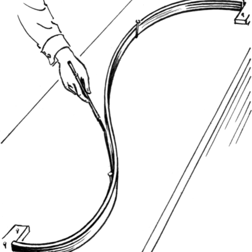
– termspline come from pre-computer (17-19. century) designers tool for creating shapes – in instruments design (violin, piano..), ship building (left pics)…
B-spline term was coined by Jacob Schoenberg (in 20. century) as short forBasic Spline. In CAD etc. it refers to piecewise polynomial (parametric) curve. Basis function term is rather used in vector based environment – meaning (generally) a function represented by set of sub-functions. In case of approximation one may rather use term blending functions.
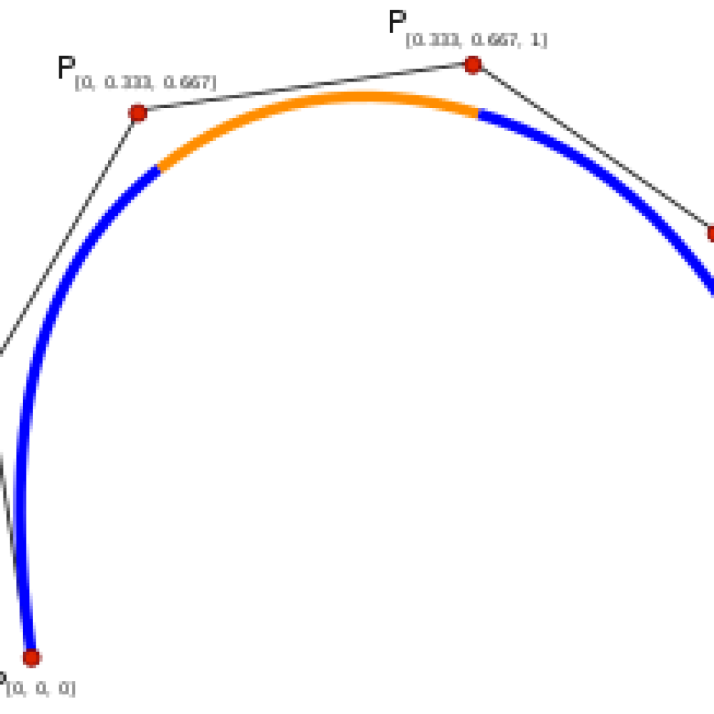
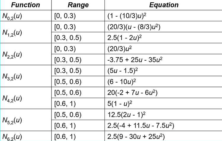
Piecewise (right pic) – means that final shape function is written is parts by sub-functions valid for particular interval (pretty typical is 0-0,3-0,5-0,6-1 as control points) etc.
One of the first approximation theories using basis function were Candinal B-spline, Hermite and Berstein basis polynomials etc.: First basis function approximations.
– Cubic B-Splines looks like have edge over typical Bezier curves: advantage is that u can change the degree to change shapes (while having same control point).
1) Forms of Bezier curves
– next 5 chapters are based on vid Continuity of splines – ytb. – while forms of Bezier curves are relatively simple, they lack local control and continuity. – they can be done w/ 4 way – tough last (matrix) combine previous two.
0) Linear interpolation (LERP)
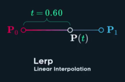
– simplest form of interpolation is 1) LERP – linear interpolation – used for lines: P(t) = (1-t)P0 + tP1 (Rpic).
– LERP is creating just lines (that why it is marked as 0 chapter), but serves as fundamental for further curves making. The LERP is actually bread and butter and w/ Brute-force and minimal amount of knowledge and objects, u should still be able to make curves…
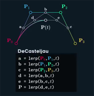
1) Decasteljau form of Bezier curve
Quadratic Bezier curves – degree 2 – is the same process of linear interpolation, but between 3 points. (Lvid)
Cubic Bezier curves (degree 3) – is one the most used form.. (vid bellow)
– are simple, but intensive on calculation. – it is basically nested recursive LERPing.
1b) Brutalist-minimalist aproachment to Decasteljau formof Bezier curve
–
– “as already said: Decasteljau crvs. are simple, but intensive on calculation.” Where else could Brutalist/ Minimalist start? – as also mentioned in the beginning, time is rather fixed domain, which restrict x, y coordinates… Time/ Level can be measured as offset from x = 1 – where Time and Level linearly from 0 approaching 1. U set time as determine/ Master, and Level as offset from linear trajectory. Ex: in 0.25 time, u want to have
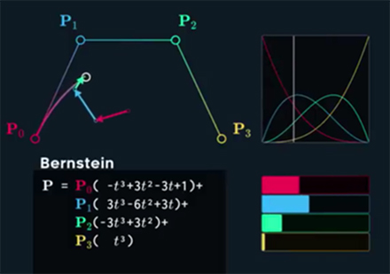
2) Berstein form of Bezier curve
– Berstein polynomials were used as a proof of Weierstrass Approximation Theorem in 1912.))
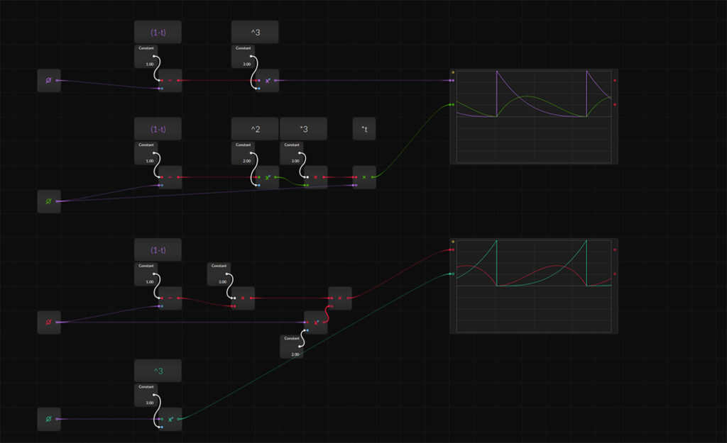
– are more effective on calculation: vectors representing each point are scaled by own cubic polynomial and add all up. These polynomial have weighting sum – convex combination: all polynomial are adding to 1 for all t values) – in the beginning 1st point have most influence (see vid).
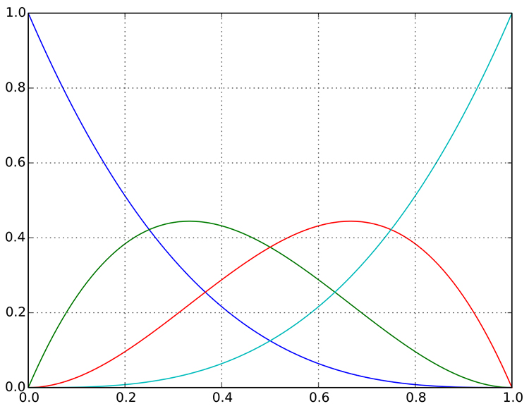
blue: y = (1 − t)3 green: y = 3(1 − t)2t red: y = 3(1 − t)t2 cyan: y = t3
This is typical approximation, based on t (time) represented by phase in Bitwig, or normalized 0-1ish ramp in Pd.
Bernstein polynomials approximating a curve:
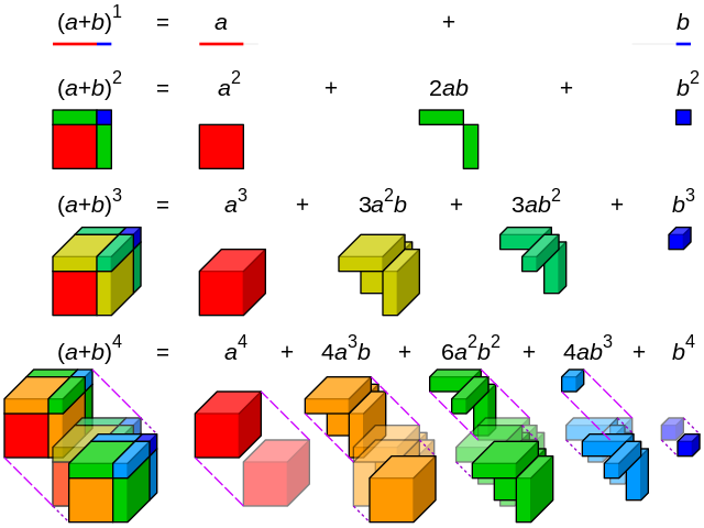
Reminder ??????????????? Polynomial probably mean any-nomial. Mononomial – single expressed term. Binominal coefficient – probably second line in Rpic: exponents share single power. Visualisation of binomial expansion up to the 4th power. (Rpic) ??????????
Lorem ipsum dolor sit amet, consectetur adipiscing elit. Ut elit tellus, luctus nec ullamcorper mattis, pulvinar dapibus leo.
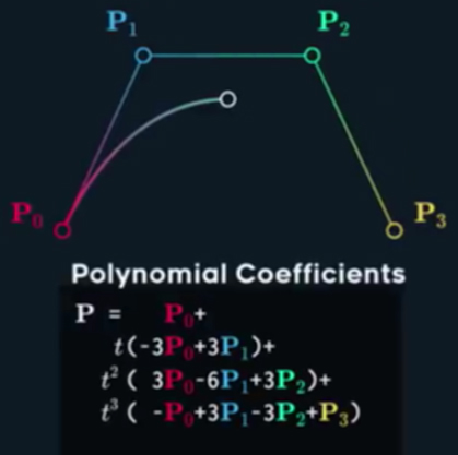
3) Polynomial coefficient form of Bezier curve
– are efficient, cause t, t^2 and t^3 are isolated, but quite complicated.
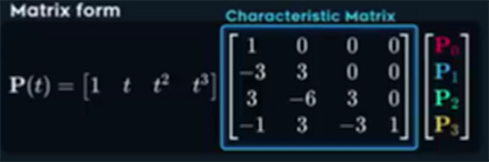
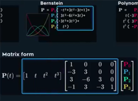
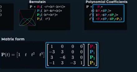
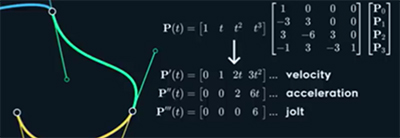
4) Matrix form
– matrix form is combination of Berstein and polynomial coefficient: – multiplying characteristic matrix by t point one gets Berstein matrix. – multiplying characteristic matrix w/ control point, one gets polynomial coefficient form.
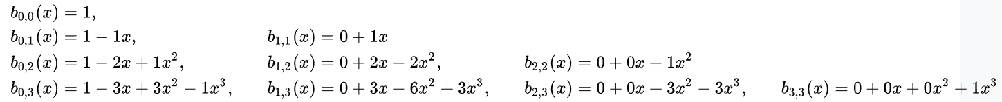
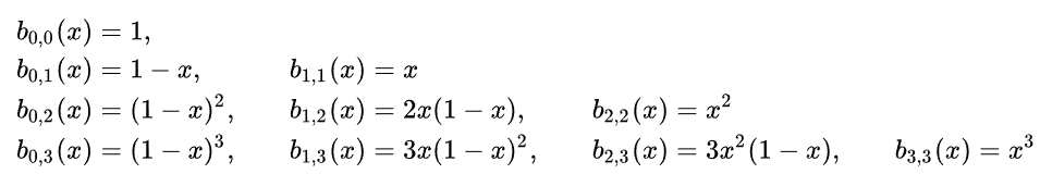
– it should be clear that if u get rid of brackets in: blue: y = (1 − t)3 green: y = 3(1 − t)2t red: y = 3(1 − t)t2 cyan: y = t3 u get marked Berstein t polynomials (Mid-pic).
Particular row of Berstein polynomials (bellow) actually represent values in column of Characteristic matrix in Matrix form (Lpic above). P0 (− t3 + 3t2 –3t P1 ( 3t3 – 6t2+ 3t P2 ( –3t2 + 3t2 P3 (t3)
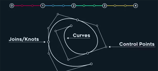
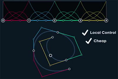
2) Form of Bezier splines
– advantage of forms of bezier splines is local control. – instead of t is traditionally used u – since it is adding more t together: integer define row and decimals particular local t value for the row. So principal is basically same, just stacking/ repeating and bit expanding previous stuff..
– Knot values are here uniform splines: each Knot interval = 1. Parametric space (Rpic) is than defined by basis fncts (L1pic bellow).
L1pic: parameters space with particular basis functions.
L2-3pics: L2 pic have range of 1 interval, L3 is twice long, but still w/ local control. L4pic: Is showing that point on line is passing thru every 3rd point. (13´).
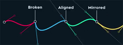
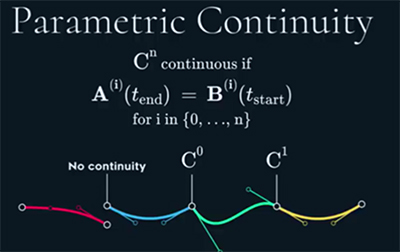
Lpic: Knots/ jointhave often so called tangents points w/ 3 basic configuration: 1) Split or Broken – first knot in pic bellow (two secondary point are not in-line – broken: defining C0 continuity). 2) Alling (two secondary point are not in-line: defining G1 continuity – see vid bellow.). 3) Mirrored – values are same in both directions (C1 continuity).
3) Continuity (C3)
– their advantage is having local control and some continuity, which in C2 level losing its usability.. which is completely is lost in C3. – continuity generally measure how line are connected.
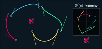
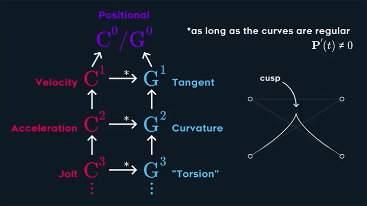
– particular value of continuity is defined by derivation – can be easily calculated from matrix from by differentiating t matrix using Power rule (Lpic): 1st derivate is Velocity (C1 continuity), 2nd derivate is Acceleration (C2) and 3rd derivation is jolt (C3).
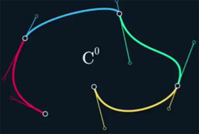
C0 continuity
– condition/ constrain of C0 continuity: points on curve are shared – connected: Red is A line, Blue is B line – lines are separated by shared P3 point.
– while C0 cont. is continuous in visual – in its position (Lpic), in 1st derivate one can see discontinuity (R1-2pics).
C1 continuity – Velocity
– condition/ constrain of C1 continuity: continuity in its position and 1st derivate called velocity.
– in Lpic one can see, that this is achieved when control point are mirrored.
– Mirroring control point on curve is actually done on every third point that divides two lines: So P3 have to have mirrored P2 and P4.
So velocity in the end of A line has to be equal to starting velocity in B line: A´(1) = B´(0) and that is P4 = 2P3 – P2. While C1 is continuous in 1st derivate (velocity), it has discontinuity in 2nd derivate (acceleration). LPic – demonstrate that changing tangent points from mirrored to broken change velocity continuity to vel. discontinuity. Rpic – demonstrating discontinuity in Acceleration.
C2 continuity
– condition/ constrain of C2 continuity: continuity in its position and 1st derivate called velocity and 2nd derivate – acceleration –
– while C2 continuity is very smooth, the constrain leads to lose of local control – what was its purpose. – again velocity in the end of A line has to be equal to starting velocity in B line: A´´(1) = B´´(0) and that is P5 = P1 + 4(P3-P2). (21´) – in 12 points only P0-1-2-3-6-9-12 points remain free – local control is lost.
C3 continuity
– constrains for C3 continuity are far beyond regular usability: A´(1) = B´(0): P6 = P3 + (P3 – P0) + 6(P1 – P2 + P3 – P2)
– from 12 points only P0-1-2-3 points remain free – local control is completely lost: it actually not even spleen, but curve (A line) extended with its extrapolation t beyond 1.
– while simple C continuity get quickly beyond its usability w/ its lost of local control, things gets better, when Geometric continuity (G) is taken into account.
– Parametric continuity: C1 is made by Mirrored tangent points, C0 w/ Broken tang. p. and no continuity if point are not connected. –
– Tangent vector (T-red) is get by normalizing the velocity vector – forcing it to have length 1 and Normal vector (green) helping here to visualize geometric G1 geometric continuity. (LPic)
– in order to understand geometric continuity (G2)– one needs to add 3rd dimension and watch (perfectly reflecting) surface for its reflections (Rpic above) – specially for reflection of lines and dots (Lpic bellow) – that is why G2 cont. is important in industrial design of shiny things like cars, phones shapes – because they are to a certain limit reflective.
But even these circle arc join only w/ G1 continuity – disorder in reflection is even more noticeable with line coming to circle curve (Rpic): from green – normalized tangent vector, and red – tangent direction, one can see This not that surprising when realize, that on circle arc angle is changing in constant speed vs. Flat line – angle is not changing at all.
For analyzing this curvature continuity in regard to circle is useful osulatingcircle (Lpic) – from Latin (Kissing circle) – describing curve curvature at particular point (Lpic). Radius of the circle is 1/k (curvature). k = |Px´ Px´´| / ||P´||^3 (see in Rpic) |Py´ Py´´| – Px and Py part is called 2D cross product
One can see (from Lpic) that it is possible to have curvature continuity even w/ C0 continuity, while C1 continuity does not guarantee having curvature continuity.
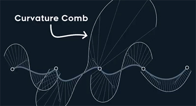
– Similarly useful for analyzing curvature continuity is curvature comb (Lpic) – cc is larger as the curvature is bigger.
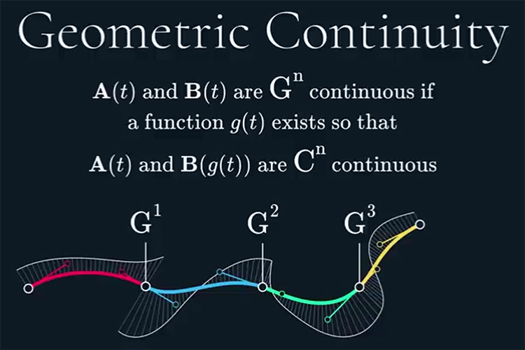
4) Geometric Continuity (G3)
Lorem ipsum dolor sit amet, consectetur adipiscing elit. Ut elit tellus, luctus nec ullamcorper mattis, pulvinar dapibus leo.
–
C0 and G0 – are both just position continuous (simple connected curve). C1 velocity to C3Joltcontinuity require having all previous level continuity (So C3 continuity implies C1 and C2 continuity). Similarly G1 Tangent to G3 Torsion requires having all previous level of geometric continuity (So G3 continuity implies G1 and G2 continuity). *applies as long as the curve is regular –
5) Further splines and finally B-spline
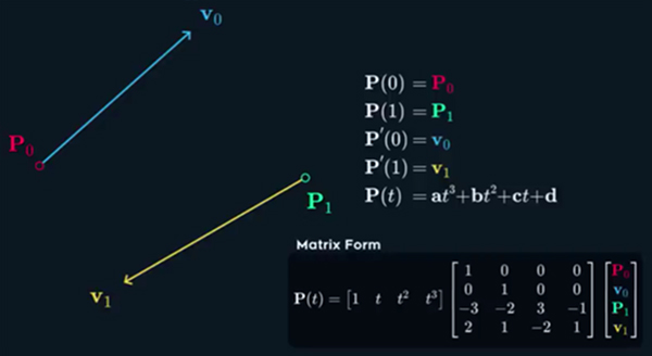
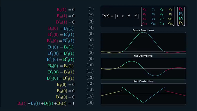
– Bezier curves define only starting and ending points, but one can also define start and end of velocity – such a spline automatically guarantee velocity continuity.
– P0 – starting point should be 0. P1 – ending point should be 1. v0 – velocity on start should be0. v1 – velocity in the end should be 1. 4 equation require 4 unknown variable – cubic polynomial Pt. Repeat: left part of matrix form is t matrix, center is Characteristic matrix and left part is point matrix. Multiplying characteristic matrix by t matrix will get point matrix.
–
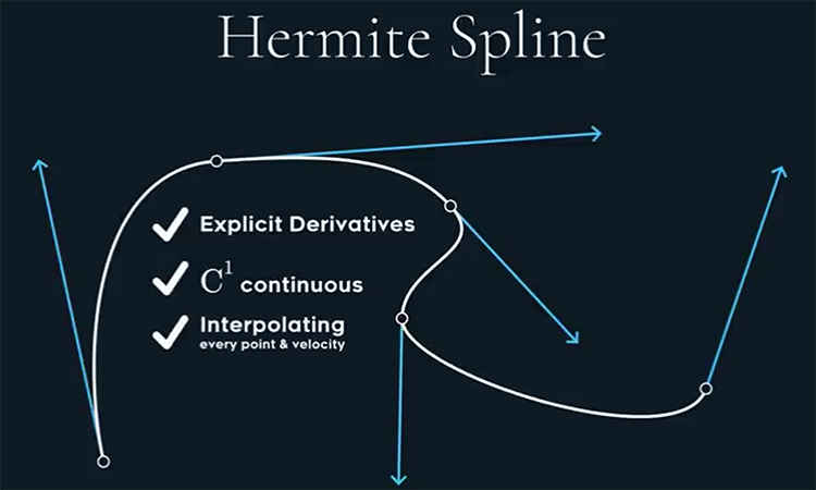
Hermite spline
– generalized Lagrange polynomials in 1864, but used also La Place concept (1810). Similar ideas also published Chebyshev (1859). – Hermite spline should be pronounce hermite, but is regularly pronounce like hermajt spline)).
–
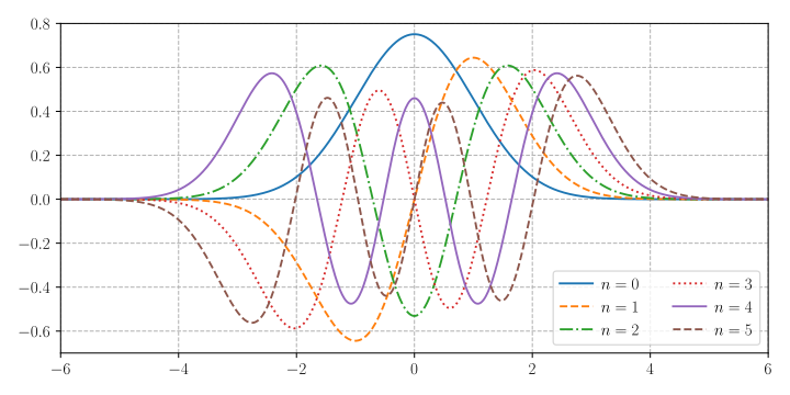
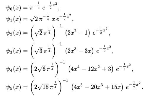
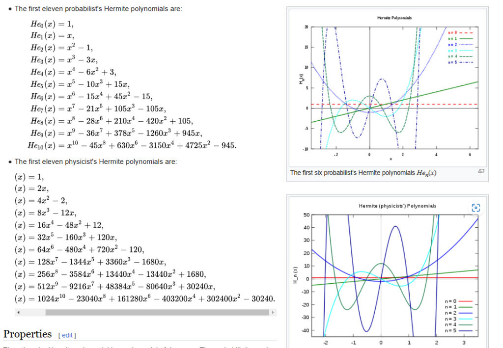
L: Schroendiger equation
As seen bellow, these polynomials are not optimize to x,y 1:1 values and probably not parametric, but either way hard to use in the Grid. Bellow are probabilistic and physic polynomials:
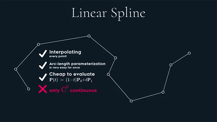
Linear spline
–
– while it is bloody limited, it has some special use – in Plug Data f. e. for ADSR line, which can be then bend.
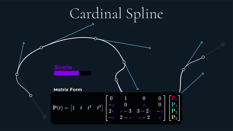
Cardinal Spline
–
–
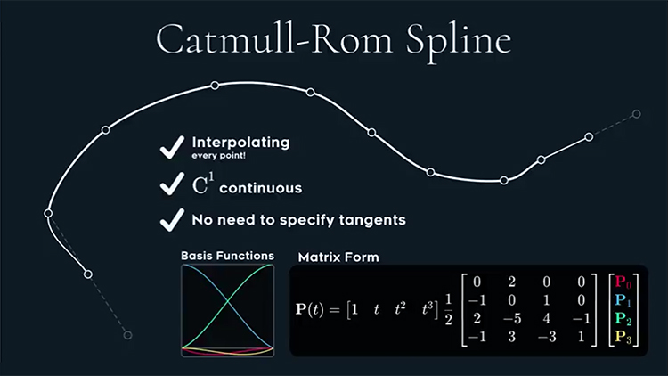
Catmull-Rom Spline
–
–
B-spline
– next chpt.
B-spline
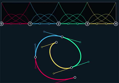
-while each type of spline have its use, B-spline (B stands for basis) looks like having edge for automation type of modulation, cause they have decent local control, while also keeping decent smoothness (C2G2). – they also have special use for smooth camera glides. – B-splines are C2 continuous – its C2 continuity was gain by giving up interpolation – B-splines are actually approximating.
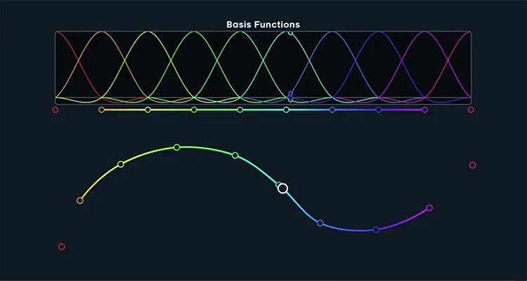
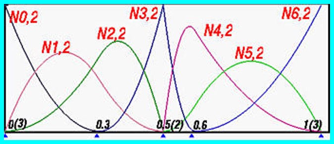
B-spline example
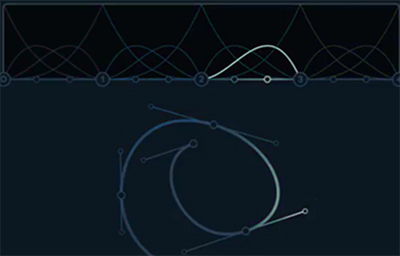
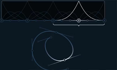
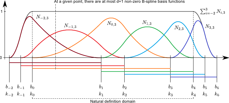
From one perspective cool is, that each function weigh influence range only to the range of its neighbor and is falling into 4th curve: 1 to 4, 2 to 5, 3 to 6. U still can change their range by Phase etc., but their end points will always stay in that value – making sure fnct. is continuous.
For some reason if multiplication of second to last is dived by two: 6,25*(————) 1,25(——————-) and in last it is devided by 10: 0,25(—————–) .. then it looks like match. But maybe I missed smth.
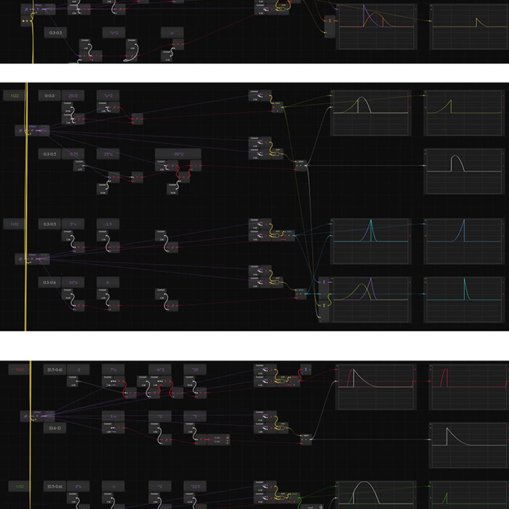
B-spline in Bitwig
As you can see, it is time consuming and options to alter polynomials in the Grid are quite limited and u can not (practically) change the degree. One is generally better off output curves from MATLAB (or other soft) into array or wavetable modules with more degrees and play with weighting … but u can do it in the Grid for first tests and it is not CPU intensive (just messy) so can be use here and there..
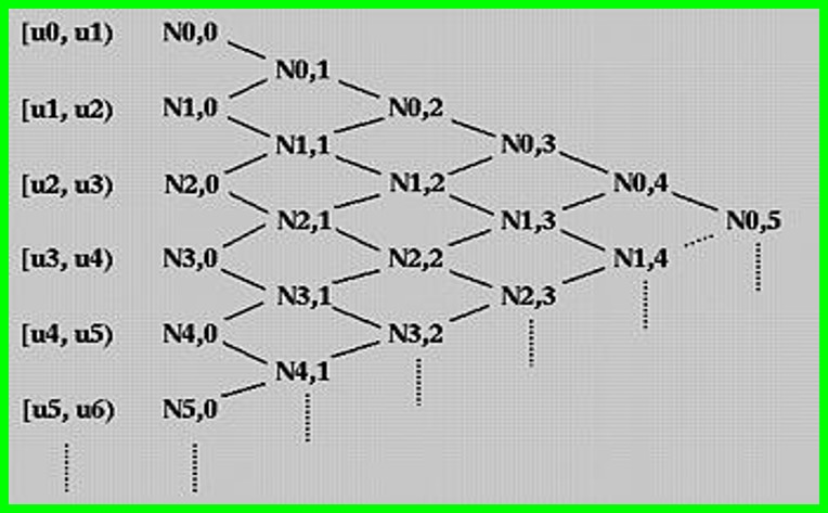
Triangular b-spline computation
Cox-de Boor recursion formula
D) Non-uniform rational basis spline (NURBS)
Sources
D. F. Roggers, J. A. Adams: Mathematical elements for computer graphics